Why did I want to read it?
What did I get out of it?
1. Introduction to Apache Spark: A Unified Analytics Engine
The “origins” of big data computing in four papers:
- The Google File System (GFS), 2003 → The Hadoop Distributed File System, 2010.
- MapReduce: Simplified Data Processing on Large Clusters, 2004.
- BigTable: A Distributed Storage System for Structured Data, 2006 which, according to Big Data and Google’s Three Papers I - GFS and MapReduce | Bowen’s blog, have only two real innovative ideas:
-
- HDFS itself.
-
- Moving computation to data (the rest of Map Reduce is just an “old programming paradigm”).
Spark address the shortcomings of Hadoop MapReduce: operational complexity, better APIs unifying different workloads, split of storage and compute, and in-memory storage of intermediate results, which Hadoop MR didn’t have and made it slow (p. 3).
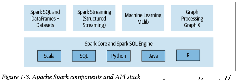
Spark convert this into a DAG that is executed by the core engine (…) the underlying code is decomposed into highly compact bytecode that is executed in the workers’ JVMs across the cluster (p. 7
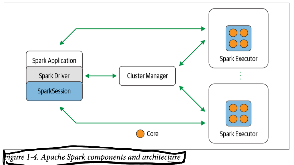
SparkSession is the API, Spark Driver requests resources from Cluster Manager and transforms Spark operations into DAG, schedules them and distributes them across the executors.
2. Getting Started
Spark Application Concepts
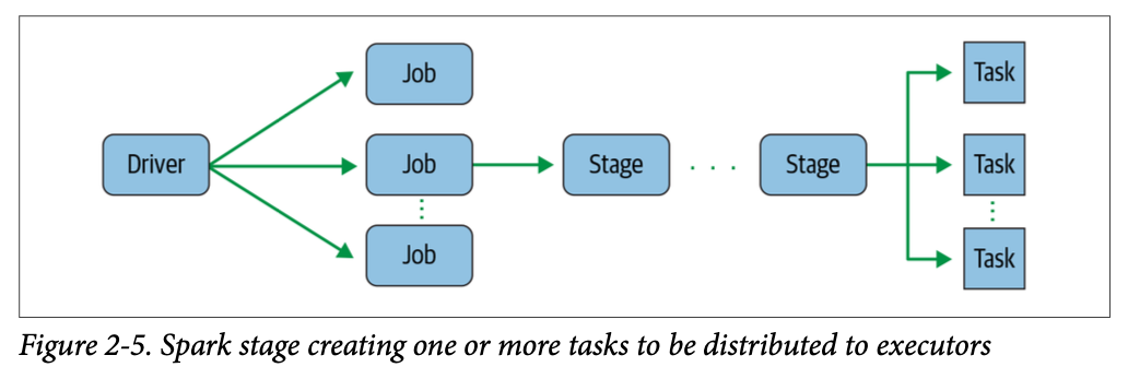
Spark transformations have lazy evaluation. A job is created whenever an action triggers a computation evaluation, e.g., a collect() (lazy evaluation). The job is transformed into a DAG. Stages are DAG nodes, based on what can be done in parallel or serially. A stage is broken down into tasks, so that each task works on a single core and single partition of data. (p. 28)
Narrow and Wide Transformations.
- Narrow: a single output partition can be computed from a single input partition (e.g., filter()).
- Wide: you need to read data from other partitions, a shuffle (e.g., groupBy, orderBy).
What if you want to use a Scala version of this same [PySpark] program? The APIS are similar; in Spark, parity is well preserved across the supported languages (p. 39).
3. Apache Spark’s Structured APIs
What’s Underneath an RDD?
RDD: Resilient Distributed Dataframe (RDDs paper). It’s an abstraction with:
- Input + list of dependencies on how the RDD is built → can be reproduced → resiliency.
- Partitions → parallelization.
- A compute function.
Structuring Spark
From, Spark 2.x, it offers an API on top of RDDs so you no longer need to work directly with them, and allowed optimizations (working with the RDDs directly not only was less readable, Spark did not know anything about the compute functions and couldn’t optimize anything).
As in Pandas, you have better performance when reading CSVs if you specify the schema (p. 58).
The Dataset API
Only makes sense in Java an Scala (although I wonder why it cannot play along with Python mypy):
Conceptually, you can think of a DataFrame in Scala as an alias for a collection of generic objects, Dataset[Row], where a Row is a generic untyped JVM object that may hold different types of fields. (p. 69)
Their only advantage is typing, because you pay a performance cost.
If you want space and speed efficiency, use DataFrames. (p. 75)
Spark SQL and the Underlying Engine
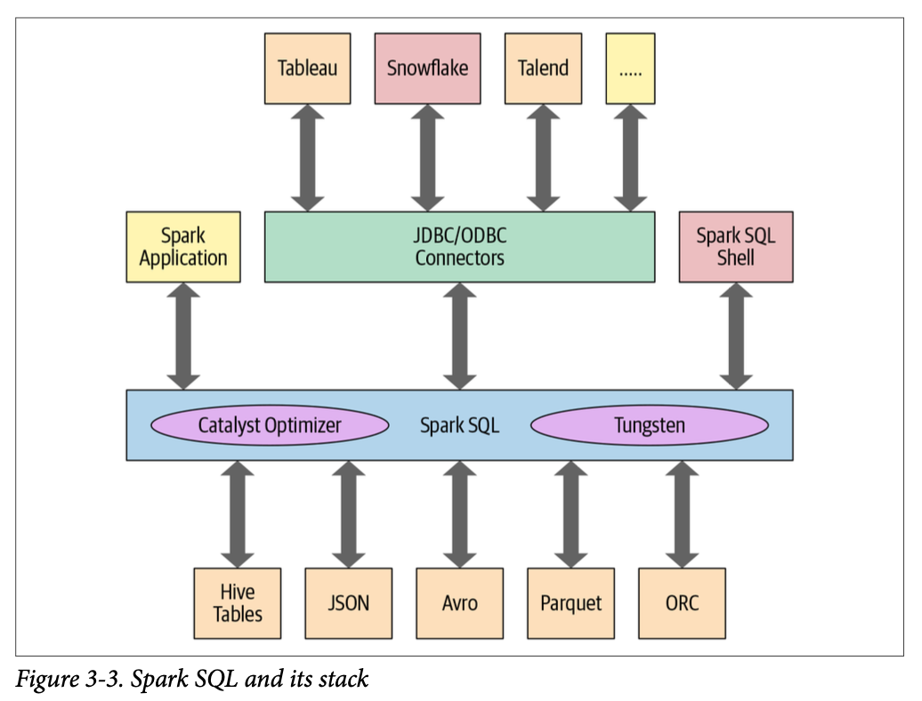
Catalyst Optimizer
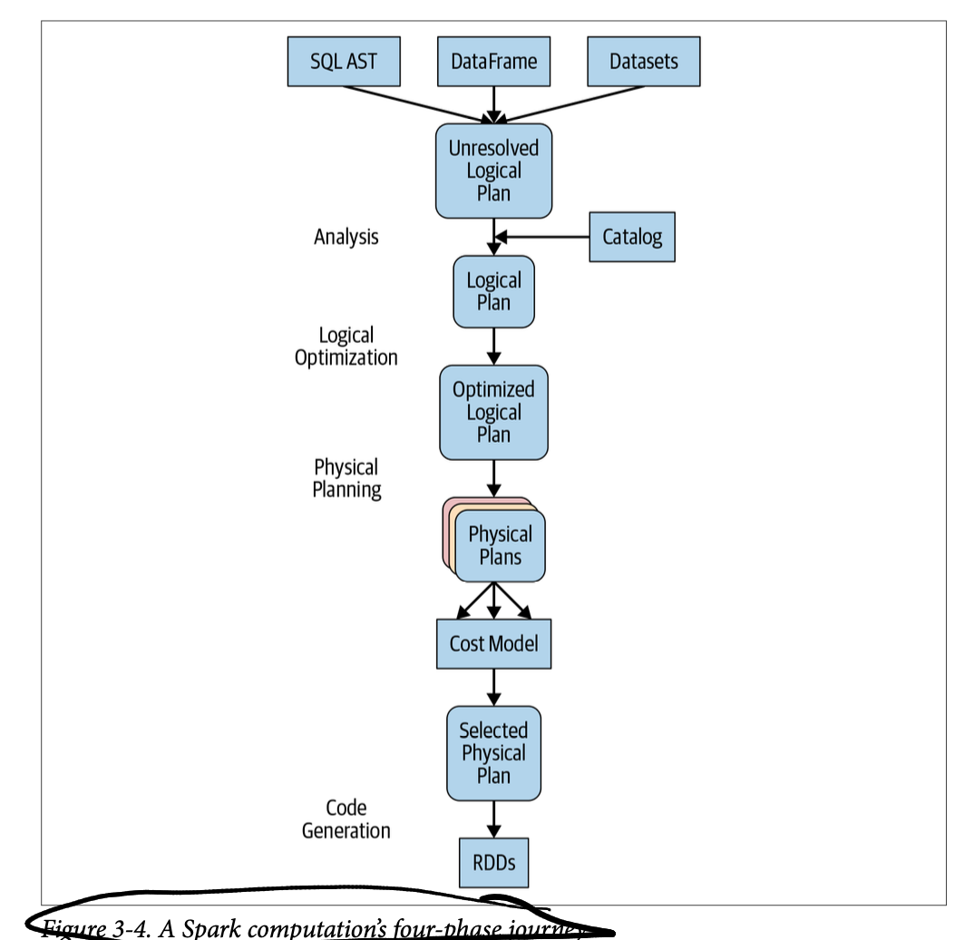
- The logical optimization has a cost-based optimizer (Cost Based Optimizer in Apache Spark 2.2 - The Databricks Blog) and it’s where magic such as predicate pushdown happens.
- The codegen phase:
It’s a physical query optimization phase that collapses the whole query into a single function, getting rid of virtual function calls and employing CPU registers for intermediate data. The second-generation Tungsten engine, introduced in Spark 2.0, uses this approach to generate compact RDD code for final execution. This streamlined strategy significantly improves CPU efficiency and performance.
So Tungsten is a compiler. See Apache Spark as a Compiler Joining a Billion Rows Per Second on a Laptop.
7. Optimizing and Tuning Spark Applications
Joins
Broadcast Hash Join
The typical were the smaller dataset is sent to all executors. Used by default if data is less than 10 MB, but can be forced (as long as you have memory on the executors… e.g., up to 100 MB).
Shuffle Sort Merge Join
Equi-joins over two large datasets with matching sortable keys. What happens is: 1. Sort of each datasets by the joining key (with a shuffle/exchange operation), 2. The join of each row on every partition. You may safe yourself from the shuffle if you store the data already sorted, with bucketing.
TODO: read more on bucketing.